

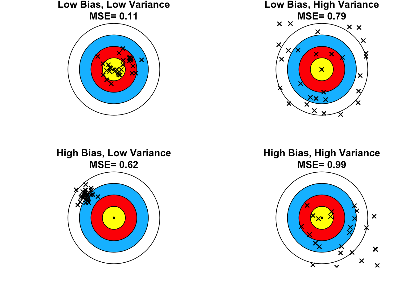

If you study enough econometrics or statistics, you’ll eventually hear someone mention “Stein’s Paradox” or the “James-Stein Estimator” . You’ve probably learned in your introductory econometrics course that ordinary least squares (OLS) is the best linear unbiased estimator (BLUE) in a linear regression model under the Gauss-Markov assumptions. The stipulations “linear” and “unbiased” are crucial here. If we remove them, it’s possible to do better–maybe even much better –than OLS. 1 Stein’s paradox is a famous example of this phenomenon, one that created much consternation among statisticians and fellow-travelers when it was first pointed out by Charles Stein in the mid-1950s. The example is interesting in its own right, but also has deep connections to ideas in Bayesian inference and machine learning making it much more than a mere curiosity. The supposed paradox is most simply stated by considering a special case of linear regression–that of estimating multiple unknown means. Efron & Morris (1977) introduce the basic idea as follows: A baseball player who gets seven hits in 20 official times at bat is said to have a batting average of .350. In computing this statistic we are forming an estimate of the player’s true batting ability in terms of his observed average rate of success. Asked how well the player will do in his next 100 times at bat, we would probably predict 35 more hits. In traditional statistical theory it can be proved that no other estimation rule is uniformly better than the observed average. The paradoxical element in Stein’s result is that it sometimes contradicts this elementary law of statistical theory. If we have three or more baseball players, and if we are interested in predicting future batting averages for each of them, then there is a procedure that is better than simply extrapolating from the three separate averages. Here “better” has a strong meaning. The statistician who employs Stein’s method can expect to predict the future averages more accurately no matter what the true batting abilities of the players may be. I first encountered Stein’s Paradox in an offhand remark by my PhD supervisor. I dutifully looked it up in an attempt to better understand the point he had been making, but lacked sufficient understanding of decision theory at the time to see what the fuss was all about. The second time I encountered it, after I knew a bit more, it seemed astounding: almost like magic. I decided to include the topic in my Econ 722 course at Penn, but struggled to make it accessible to my students. A big problem, in my view, is that the proof–see lecture 1 or section 7.3 –is ultimately a bit of a let-down: algebra, followed by repeated integration by parts, and then a fact about the existence of moments for an inverse-chi-squared random variable . It seems like a sterile technical exercise when in fact that result itself is deep, surprising, and important. As if a benign deity were keen on making my point for me, the wikipedia article on the James-Stein Estimator is flagged as “may be too technical for readers to understand” at the time of this writing! After six months of pondering, this post is my attempt to explain the James-Stein Estimator in a way that is accessible to a broad audience. The assumed background is minimal: just an introductory course probability and statistics. I’ll show how we can arrive at something that is very nearly the James-Stein estimator by following some very simple and natural intuition. After you understand my “not quite James-Stein” estimator, it’s a short step to the real thing. So the “let-down” proof I mentioned before becomes merely a technical justification for a slight modification of a formula that is already intuitively compelling. As far as possible, I’ve tried to keep this post self-contained by introducing, or at least reviewing, key background material as we go along. The cost of this approach, unfortunately, is that the post is pretty long! I hope you’ll soldier on the the end and that you’ll find the payoff worth your time and effort. As far as I know, the precise way that I motivate the James-Stein estimator in this post is new, but there are are many other papers that aim to make sense of the supposed paradox in an intuitive way. In keeping with my injunction that you should always consider reading something else instead , here are a few references that you may find helpful. Efron & Morris (1977) is a classic article aimed at the general reader without a background in statistics. Stigler (1988) is a more technical but still accessible discussion of the topic while Casella (1985) is a very readable paper that discusses the James-Stein estimator in the context of empirical Bayes. A less well-known paper that I found helpful is Ijiri & Leitch (1980) , who consider the James-Stein estimator in a real-world setting, namely “Audit Sampling” in accounting. They discuss several interesting practical and philosophical issues including the distinction between “composite” and “individual” risk that I’ll pick up on below. Warm-up Exercise This section provides some important background that we’ll need to understand Stein’s Paradox later in the post reviewing the ideas of bias , variance and mean-squared error along with introducing a very simple shrinkage estimator . To make these ideas as transparent as possible we’ll start with a ridiculously simple problem. Suppose that you observe (X \sim \text{Normal}(\mu, 1)) , a single draw from a normal distribution with variance one and unknown mean (\mu) . Your task is to estimate (\mu) . This may strike you as a very silly problem: it only involves a single datapoint and we assume the variance of (X) is one! But in fact there’s nothing special about (n = 1) and a variance of one: these merely make the notation simpler. If you prefer, you can think of (X) as the sample mean of (n) iid draws from a population with unknown mean (\mu) where we’ve rescaled everything to have variance one. So how should we estimate (\mu) ? A natural and reasonable idea is to use the sample mean, in this case (X) itself. This is in fact the maximum likelihood estimator for (\mu) , so I’ll define (\hat{\mu}{\text{ML}} = X) . But is this estimator any good? And can we find something better? Review of Bias, Variance and MSE The concepts of bias and variance are key ideas that we typically reach for when considering the quality of an estimator. To refresh your memory, bias is the difference between an estimators expected value and the true value of the parameter being estimated while variance is the expected squared difference between an estimator and its expected value. So if (\hat{\theta}) is an estimator of some unknown parameter (\theta) , then (\text{Bias}(\hat{\theta}) = \mathbb{E}[\hat{\theta}] - \theta) while (\text{Var}(\hat{\theta}) = \mathbb{E}[(\hat{\theta} - \mathbb{E}[\hat{\theta}])^2]) . A bias of zero means that an estimator is correctly centered : its expectation equals the truth. We say that such an estimator is unbiased . 2 A small variance means that an estimator is precise : it doesn’t “jump around” too much. Ideally we’d like an estimator that is correctly centered and precise. But it turns out that there is generally a trade-off between bias and variance: if you want to reduce one of them, you have to accept an increase in the other. A common way of trading off bias and variance relies on a concept called mean-squared error (MSE) defined as the sum of the squared bias and the variance. 3 In particular: (\text{MSE}(\hat{\theta}) = \text{Var}(\hat{\theta}) + \text{Bias}(\hat{\theta})^2) . Equivalently, we can write (\text{MSE}(\hat{\theta}) = \mathbb{E}[(\hat{\theta} - \theta)^2]) . 4 To borrow some terminology from introductory microeconomics, you can think of MSE as the negative of a utility function over bias and variance. Both bias and variance are “bads” in that we’d rather have less rather than more of each. This formula expresses our preferences in terms of how much of one we’d be willing to accept in exchange for less of the other. Slightly foreshadowing something that will come later in this post, we can think of MSE as the square of the average distance that an archer’s arrows land from the bulls-eye. Smaller values of MSE are better: variance measures how closely the arrows cluster together while bias measures how far the center of the cluster is from the bulls-eye, as in the following diagram: A Shrinkage Estimator Returning to our maximum likelihood estimator: it’s unbiased, (\text{Bias}(\hat{\mu}{\text{ML}}) = 0) , so (\text{MSE}(\hat{\mu}{\text{ML}}) = \text{Var}(\hat{\mu}{\text{ML}}) = 1) . Suppose that low MSE is what we’re after. Is there any way to improve on the ML estimator? In other words, can we achieve an MSE that’s lower than one? The answer turns out to be yes . Here’s the idea. Suppose we had some reason to believe that the true mean (\mu) isn’t very large. Then perhaps we could try to adjust our maximum likelihood estimate by shrinking slightly towards zero. One way to do this would be by taking a weighted average of the ML estimator and zero: [ \hat{\mu}(\lambda) = (1 - \lambda) \times \hat{\mu}{\text{ML}} + \lambda \times 0 = (1 - \lambda)X ] for (0 \leq \lambda \leq 1) . The constant ((1 - \lambda)) is called the “shrinkage factor” and controls how the ML estimator gets pulled towards zero. 5 We get a different estimator for every value of (\lambda) . If (\lambda = 0) then we get the ML estimator back. If (\lambda = 1) then we get a very silly estimator that ignores the data and simply reports zero no matter what! So let’s see how the MSE depends on our choice of (\lambda) . Substituting the definition of (\hat{\mu}(\lambda)) into the formulas for bias and variance gives: [ \begin{align*} \text{Bias}[\hat{\mu}(\lambda)]&= \mathbb{E}[(1 - \lambda)\hat{\mu}\text{ML}] - \mu = (1 - \lambda)\mathbb{E}[\hat{\mu}\text{ML}] - \mu = (1 - \lambda)\mu - \mu = -\lambda\mu\ \ \text{Var}[\hat{\mu}(\lambda)]&= \text{Var}[(1 - \lambda)\hat{\mu}\text{ML}] = (1 - \lambda)^2\text{Var}[\hat{\mu}_\text{ML}] = (1 - \lambda)^2\ \ \text{MSE}[\hat{\mu}(\lambda)]&= \text{Var}[\hat{\mu}(\lambda)] + \text{Bias}[\hat{\mu}(\lambda)]^2 = (1 - \lambda)^2 + \lambda^2\mu^2 \end{align*} ] Unless (\lambda = 0) , the shrinkage estimator is biased . And while the MSE of the ML estimator is always one, regardless of the true value of (\mu) , the MSE of the shrinkage estimator depends on the unknown parameter (\mu) . So why should we use a biased estimator? The answer is that by tolerating a small amount of bias we may be able to achieve a larger reduction in variance, resulting in a lower MSE compared to the higher variance but unbiased ML estimator. A quick plot shows us that the shrinkage estimator can indeed have a lower MSE than the ML estimator depending on the value of (\lambda) and the true value of (\mu) : # Range of values for the unknown parameter mu mu <- seq(-4, 4, length = 100)
Try three different values of lambda
lambda1 <- 0.1 lambda2 <- 0.2 lambda3 <- 0.3
Plot the MSE of the shrinkage estimator as a function of mu for all
three values of lambda at once
matplot(mu, cbind((1 - lambda1)^2 + lambda1^2 * mu^2, (1 - lambda2)^2 + lambda2^2 * mu^2, (1 - lambda3)^2 + lambda3^2 * mu^2), type = 'l', lty = 1, lwd = 2, col = c('red', 'blue', 'green'), xlab = expression(mu), ylab = 'MSE', main = 'MSE of Shrinkage Estimator')
Add legend
legend('topright', legend = c(expression(lambda == 0.1), expression(lambda == 0.2), expression(lambda == 0.3)), col = c('red', 'blue', 'green'), lty = 1, lwd = 2)
Add dashed line for MSE of ML estimator
abline(h = 1, lty = 2, lwd = 2) Some Algebra It’s time for some algebra. If you’re tempted to skip this please don’t : this section is a warm-up for our main event. If you thoroughly understand the mechanics of shrinkage in this simple example, everything that follows below will seem much more natural. As seen from the plot above, the MSE of our shrinkage estimator (the solid lines) is lower than that of the ML estimator (the dashed line) provided that our chosen value of (\lambda) isn’t too large relative to the true value of (\mu) . With a bit of algebra, we can work out precisely how large (\lambda) can be to make shrinkage worthwhile. Since (\text{MSE}[\hat{\mu}\text{ML}]= 1) , by expanding and simplifying the expression for (\text{MSE}[\hat{\mu}(\lambda)]) we see that (\text{MSE}[\hat{\mu}(\lambda)] < \text{MSE}[\hat{\mu}\text{ML}]) if and only if [ \begin{align*} (1 - \lambda)^2 + \lambda^2\mu^2 &< 1 \ 1 - 2\lambda + \lambda^2 + \lambda^2\mu^2 &< 1 \ \lambda^2 (1 + \mu^2) -2 \lambda &< 0 \ \lambda [\lambda (1 + \mu^2) - 2] &< 0. \end{align*} ] Since (\lambda \geq 0) , the final inequality can only hold if the factor inside the square brackets is negative, i.e. [ \begin{align*} \lambda (1 + \mu^2) - 2 &< 0 \ \lambda &< \frac{2}{1 + \mu^2}. \end{align*} ] This shows that any choice of (\lambda) between (0) and (2 / (1 + \mu^2)) will give us a shrinkage estimator with an MSE less than one. To check our algebra, we can change the inequality to an equality and solve for (\mu) to obtain the boundary of the region where shrinkage is better than ML: [ \begin{align*} \lambda (1 + \mu^2) - 2 &= 0 \ 1 + \mu^2 &= 2/\lambda \ \mu &= \pm \sqrt{2/\lambda - 1}. \end{align*} ] Adding these boundaries to a simplified version of our previous plot with only (\lambda = 0.3) we see that everything works out correctly: the dashed red lines intersect the blue curve at the points where the MSE of the shrinkage estimator equals that of the ML estimator. # Plot the MSE of the shrinkage estimator as a function of mu for lambda = 0.3 lambda <- 0.3 plot(mu, (1 - lambda)^2 + lambda^2 * mu^2, type = 'l', lty = 1, lwd = 2, col = 'blue', xlab = expression(mu), ylab = 'MSE', main = 'Boundary of Region Where Shrinkage is Better than ML')
Add dashed line for MSE of ML estimator
abline(h = 1, lty = 2, lwd = 2)
Add boundaries of region where shrinkage is better than ML estimator
abline(v = c(sqrt(2/lambda - 1), -sqrt(2/lambda - 1)), lty = 3, lwd = 2, col = 'red') But there’s still more to learn! Suppose we wanted to take things one step further and find the optimal value of (\lambda) for any given value of (\mu) . In other words, suppose we wanted the value of (\lambda) that minimizes the MSE of our shrinkage estimator given a particular assumed value for (\mu) . Since (\text{MSE}[\hat{\mu}(\lambda)]) is a quadratic function of (\lambda) , as shown above, this turns out to be a fairly straightforward calculation. Differentiating, [ \begin{align*} \frac{d}{d\lambda}\text{MSE}[\hat{\mu}(\lambda)] &= \frac{d}{d\lambda}[(1 - \lambda)^2 + \lambda^2 \mu^2] \ &= -2(1 - \lambda) + 2\lambda \mu^2 \ &= 2 [\lambda (1 + \mu^2) - 1]\ \ \frac{d^2}{d\lambda^2}\text{MSE}[\hat{\mu}(\lambda)] &= 2(1 + \mu^2) > 0 \end{align*} ] so there is a unique global minimum at (\lambda^* \equiv 1/(1 + \mu^2)) . This gives the optimal shrinkage factor in the sense that it minimizes the MSE of the shrinkage estimator. Substituting (\lambda^) into the expression for (\text{MSE}[\hat{\mu}(\lambda)]) gives: [ \begin{align} \text{MSE}[\hat{\mu}(\lambda^)] &= \left(1 - \frac{1}{1 + \mu^2} \right)^2 + \left(\frac{1}{1 + \mu^2}\right)^2 \mu^2 \ &= \left( \frac{\mu^2}{1 + \mu^2}\right)^2 + \left(\frac{1}{1 + \mu^2}\right)^2 \mu^2 \ &= \left( \frac{1}{1 + \mu^2}\right)^2 (\mu^4 + \mu^2) \ &= \left( \frac{1}{1 + \mu^2}\right)^2 \mu^2(1 + \mu^2) \ &= \frac{\mu^2}{1 + \mu^2} < 1. \end{align} ] Stein’s Paradox Recap We’re moments away from having all the ingredients we need to introduce Stein’s Paradox! But first let’s review what we’ve uncovered thus far. We’ve seen that the shrinkage estimator can improve on the ML estimator in terms of MSE provided that (\lambda) is chosen judiciously: it needs to be between zero and (2/(1 + \mu^2)) . The optimal choice of (\lambda) , namely (\lambda^* = 1 / (1 + \mu^2)) , gives an MSE of (\mu^2/(1 + \mu^2)) . This is always lower than one, the MSE of the ML estimator. There’s just one massive problem we’ve ignored this whole time: we don’t know the value of (\mu) ! As seen from the figure plotted above, the MSE curves for different values of (\lambda) cross each other : the best one to use depends on the true value of (\mu) . This doesn’t mean that all is lost. Perhaps in practice we have some outside information about the likely value of (\mu) that could help guide our choice of (\lambda) . What it does mean is that there’s no “one-size-fits-all” value. Admissibility It’s time to introduce a bit of technical vocabulary. We say that an estimator (\tilde{\theta}) dominates another estimator (\hat{\theta}) if (\text{MSE}[\tilde{\theta}] \leq \text{MSE}[\hat{\theta}]) for all possible values of the parameter (\theta) being estimated and (\text{MSE}[\tilde{\theta}] < \text{MSE}[\hat{\theta}]) for at least one possible value of (\theta) . 6 In words, this means that it never makes sense to use (\hat{\theta}) in preference to (\tilde{\theta}) . No matter what the true parameter value is, you can’t do worse with (\tilde{\theta}) and you might do better. An estimator that is not dominated by any other estimator is called admissible ; an estimator that is dominated by some other estimator is called inadmissible . The concept of admissibility in decision theory is a bit like the concept of Pareto efficiency in microeconomics. An admissible estimator is only “good” in the sense that it doesn’t leave any money on the table: there’s no way to do better for one parameter value without doing worse for another. In a similar way, a Pareto efficient allocation in economics is one in which no individual can be made better off without making another person worse off. It’s quite challenging to prove, but in fact the ML estimator (\hat{\theta}{ML} = X) turns out to be admissible in our little example. So while we could potentially do better by using shrinkage, it’s not a slam-dunk case. If we really have no idea of how large (\mu) is likely to be, the ML estimator is a reasonable choice. Because it’s admissible, at the very least we know that there’s no free lunch! A More General Example Now let’s make things a bit more interesting. For the rest of this post, suppose that we observe not a single draw (X) from a (\text{Normal}(\mu, 1)) distribution but a collection of (p) independent draws from (p) different normal distributions: [ X_1, X_2, ..., X_p \sim \text{independent Normal}(\mu_j, 1), \quad j = 1, ..., p. ] You can think of this as (p) copies of our original problem: we observe (X_j \sim \text{Normal}(\mu_j, 1)) and our task is to estimate (\mu_j) . The observations are all independent, and each comes from a distribution with a potentially different mean . At first glance it seems like these (p) separate problems should have absolutely nothing to do with each other . And indeed the maximum likelihood estimator for the collection of (p) means is simply (\hat{\mu}^{(j)}\text{ML} = X_j) . As above in our example with (p=1) , the question is: how good is the ML estimator, and can we do any better? Composite MSE But first things first: how can we evaluate the quality of (p) estimators for (p) different parameters at the same time ? A common approach, and the one we will follow here, is to take the sum of the individual MSEs of each estimator, yielding a quantity called composite MSE . If (\hat{\mu}_1, \hat{\mu}_2, \dots, \hat{\mu}p) is a collection of estimators for each of the individual unknown means, then the composite MSE is defined as [ \text{Composite MSE} \equiv \sum{j=1}^p \text{MSE}(\hat{\mu}j) = \sum{j=1}^p \left[ \text{Bias}(\hat{\mu}_j)^2 + \text{Var}(\hat{\mu}j)\right] = \sum{j=1}^p \mathbb{E}[(