


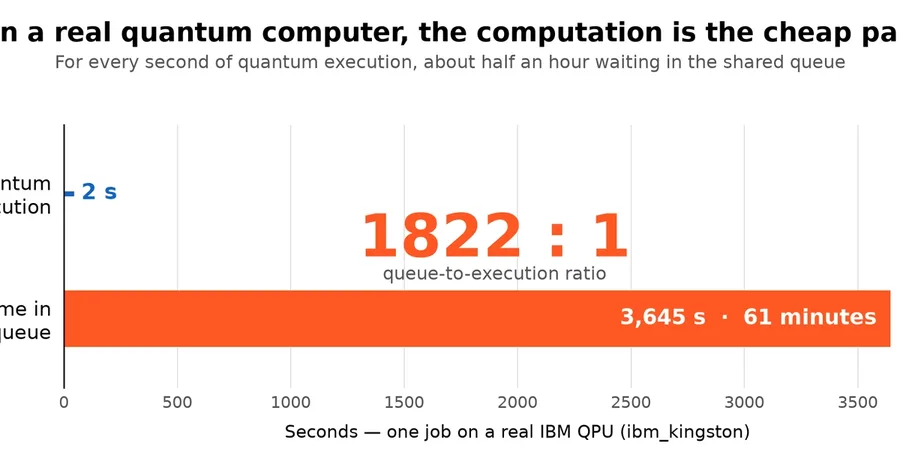
On the same IBM quantum processor, on the same afternoon, the same two-qubit circuit took 2 seconds to run and 61 minutes to reach the front of the queue — a queue-to-execution ratio of 1822:1 . For every second of actual quantum computation, the user waited more than half an hour in line. The quantum part was never the bottleneck. The scheduling was. TL;DR. Quantum computers are now cloud resources, and the literature treats their real-world friction — queue latency, backend availability, fallback, provider choice — as a qualitative footnote. I built Quantum Orchestrator , an open-source multi-provider scheduler (IBM, AWS, IonQ), and turned those footnotes into measurements. Real QPU execution is stable at ~2 s while queue time on the same machine ranges from 10 s to 61 min ( up to 1822:1 ); autonomous backend selection moves not only wait time but fidelity (~94% vs 97% on the same circuit, different processors); and a two-basis VQE reaches H₂'s ground-state energy to chemical accuracy, cleanly separating averaged-away shot noise from a fixed noise-model bias. Along the way, an external code review of the repository caught two correctness bugs that my own instrumentation had missed, and a third surfaced once I fixed them — a story I keep in, because honest instrumentation (mine and a second reader's) is part of the result. 1. Introduction — the bottleneck isn't where you think Quantum computers have mostly left the laboratory bench. You no longer walk up to a dilution refrigerator; you send a job to one, the same way you send a job to any other cloud resource. IBM, AWS, and others now expose real quantum processors behind an API and a queue — Quantum Computing as a Service. And because the machines themselves are so striking, almost all of the attention goes to the physics inside them: qubit counts, gate fidelities, error rates. My undergraduate thesis in Computer Engineering argued that this focus is misplaced. Seen from a systems-architecture angle, the hard part of using a quantum computer today is not the quantum part — it is everything around it: waiting in a shared queue, deciding which provider and which machine to send a job to, falling back to a simulator when the real device is unreachable, and knowing whether the number that comes back can be trusted. The thesis made that case in words. Like most of the literature it drew on, it never made it in numbers: every claim about queues, fallback, and backend choice was a reasonable sentence and an untested assertion. This article is what happens when you try to measure the assertion. I built Quantum Orchestrator , an open-source, multi-provider scheduler that accepts any standard quantum circuit, autonomously selects the best available backend across IBM, AWS, and IonQ, runs the job with automatic fallback, and reports fidelity, queue time, execution time, and — for a chemistry benchmark — molecular ground-state energy. Then I ran it, on real hardware and calibrated simulators, and recorded what actually happened. What happened is that the orchestration, not the computation, dominates — and in ways the platform's own numbers do not warn you about. The queue, not the quantum execution, is where the time goes. The choice of machine, not merely the wait, is where the fidelity goes. And a benchmark number that has stopped moving is trustworthy only once you separate the noise that averages away from the bias that never does. None of this required a new algorithm or a bigger quantum computer. It required treating quantum access as an engineering problem — scheduling, routing, instrumentation, honest error bars — and then measuring it. That is the argument of this piece: for the engineer, quantum computing today is an orchestration problem . The rest of this article shows the measurements that back it up, including two correctness bugs an external review caught in my own code and a third that followed from fixing them, because how you find out you were wrong is part of the result. 2. Background: a thesis claim that was never measured Reaching a quantum computer today is oddly mundane. You authenticate against a cloud platform — for IBM, a Cloud IAM key and an instance identifier now, not the old direct token — submit a circuit, and wait in a shared queue behind everyone else aimed at the same machine. There is no local install of a real QPU, no reservation, no SLA you would recognize from classical cloud computing. The device runs your job in seconds and hands back a distribution over bitstrings; everything hard happens before and after it — authentication, queueing, fallback, provider heterogeneity, and knowing whether the result can be trusted. My thesis made exactly this systems-architecture case, and — like the literature it drew on — made it entirely in words. Those claims are well rehearsed. Quantum-computing-as-a-service has been framed as a software-engineering discipline in its own right [Muhammad et al., 2025], and quantum-cloud reviews catalogue queueing, provider heterogeneity, and result validation as open problems [Nguyen et al., 2024]. A QPU may be unavailable and subject to queues. One can fall back to a simulator. A backend selector could choose the best target by availability, cost, and result quality. Every one of these is plausible. Not one was a measurement. How long is the queue, really? Does the API's own queue metric predict it? Does the choice of machine change only the wait, or the answer itself? What does falling back actually cost you in fidelity? This project exists to replace those conditionals with measurements — one assertion at a time. It is not a restatement of the thesis; it is the thesis's missing experiment. Where the thesis drew a reference architecture, this builds it and runs it; where the thesis tabulated plausible trade-offs, this reports measured ones. The rest of the article is that replacement. 3. What I built Quantum Orchestrator is a command-line tool with one job: take a quantum circuit, decide where to run it, run it, and report what happened. In practice it is a thin routing-and-observability layer between a program and a set of quantum backends — the piece that decides whether a job goes to real hardware or a simulator, waits out the queue, handles failure, and records what came back. The design rests on a single abstraction. Every backend — a local simulator, a noisy simulator, a real IBM QPU, an Amazon Braket device — implements the same small BackendAdapter interface: is it available, what is its estimated queue, run this circuit, what is your name. The orchestrator never knows which provider it is talking to; it only talks to the interface. Adding a provider means writing one adapter, nothing else. (The engineering behind that abstraction — and the one place it leaks — is Part 2.) Behind the interface sit five backends: an ideal Aer simulator (the noiseless reference), a noisy Aer simulator (a calibrated IBM-style noise model), a real IBM superconducting QPU selected autonomously at run time, an AWS Braket local simulator, and an IonQ trapped-ion simulator. I chose IonQ over Azure Quantum deliberately: Azure's local simulator needs a configured cloud workspace and would have been one more ideal simulator, whereas IonQ contributes a genuinely different physical qubit technology — trapped ions versus superconducting circuits — and therefore a different error profile to compare against. On top of the backends run three benchmark circuits of increasing depth — a Bell state (2 qubits, validation), a GHZ state (3 qubits, medium complexity), and a VQE ansatz for the H₂ molecule (2 qubits, the "real use case") — and three execution strategies, responsive , accurate , and adaptive , that decide how hard to try for the real hardware before falling back. I look at the three strategies more closely in Part 2. Everything runs on free tiers: an IBM Quantum account and local simulators, no paid cloud. That is deliberate — a measurement study nobody can reproduce is just an anecdote with graphs. Part 1 — Benchmarking the backends 4. Queue versus execution: the 1822:1 ratio I timed a real IBM run in two halves: the quantum execution, and the wait to get on the machine. Execution was boringly stable — 2 seconds on fifteen of the eighteen hardware runs in the log, and under a second on the other three, across every circuit and every IBM backend. The wait was not: on the same hardware it ran anywhere from roughly 10 seconds to just over an hour — 3,645 seconds on one ibm_kingston submission. All of the variance lived in the queue, and none of it in the computation. Three things follow from that gap, and together they are why the rest of this project exists. The platform does not expose the number you need. When I submitted that hour-long job, ibm_kingston reported a single pending job. IBM's own dashboard estimate — "Estimated QR usage: 4 s" — turned out to be accurate, and accurate about the wrong thing: it estimates quantum runtime , the execution, and execution took 2 seconds. What no number on the page predicted was the 3,645 seconds spent before that execution began. The one queue signal the API does expose, pending_jobs , was as low as it goes; reading it the obvious way — one pending job, one job's worth of waiting — underestimated the actual wait by a factor of sixty. On that same afternoon in June, ibm_fez and ibm_marrakesh , with a comparable handful of pending jobs, returned the same work in 10 to 23 seconds. pending_jobs is necessary information and nowhere near sufficient. A shared QPU is not a FIFO line. That unpredictability is not a platform bug; it is what shared quantum hardware is . Scheduling folds in priorities, calibration cycles, maintenance windows, and job characteristics invisible from the outside. You cannot reason about the wait from the single number you are handed. So the scheduler cannot trust a fixed cutoff. If the queue signal is unreliable, then deciding "give up on the hardware after N seconds" with a fixed N is guesswork. The tool instead sizes its fallback threshold in proportion to the expected execution time and caps every attempt with an absolute timeout — the mechanics are in Part 2. Put the two halves back together and the headline lands: 3,645 seconds of waiting for 2 seconds of computing — a queue-to-execution ratio of 1822 to 1. On today's quantum cloud, the computation is the cheap part. Everything expensive is the queue. (That 3,645-second wait predates the tool's current 30-minute absolute timeout, described in Part 2. Re-running this exact scenario today would have the job cancelled at 1,800 s rather than left to complete at 3,645 s — the cap exists precisely because a wait like this one is possible. The queue variability the measurement demonstrates is unaffected; the specific 1822:1 figure is a real historical measurement, not a number today's tool would let recur unbounded.) 5. Backend selection moves fidelity, not just latency The queue is the obvious reason to care which machine you land on. It is not the only one. I ran the GHZ circuit five times on real IBM hardware, letting the scheduler place each run on whatever machine had the shortest queue. The five fidelities did not scatter randomly around an average — four runs landed on ibm_fez and came back at 94.0%, 95.3%, 93.3%, and 93.3%; the one run that landed on ibm_marrakesh came back at 97.3%. The ibm_fez runs cluster tightly around 94%; the single ibm_marrakesh run sits clearly above all four of them. That reframes what a "backend selector" is for. The tool selects autonomously by the lowest reported queue — a latency decision — but the machine it picks also sets the quality of the answer, because two processors of the same generation are calibrated differently, drift differently, and carry different error rates on any given day. Choosing the shortest queue and choosing the best result are not the same choice, yet the same component makes both. This is the part of orchestration with no classical analogue. Route a job to one cloud VM instead of another and you expect the same output. Route it to one QPU instead of another and you can get a measurably different distribution — here, roughly three percentage points of fidelity — from nothing but the target. An engineer who treats all "available QPUs" as interchangeable is leaving result quality to chance. The honest limit: this is five real runs from a single session, split four and one across the machines — the scheduler's own least-busy-queue logic, not a deliberate design, is what produced that lopsided split. Four points is enough to see ibm_fez 's cluster; one point on ibm_marrakesh is a single data point, not a distribution, and I am not turning it into a mean-plus-error-bar it cannot support. What the single run does support is that on the same afternoon, on the same circuit, the two machines were not interchangeable — consistent, in direction and rough size, with the same gap seen on Bell (Section 7: ibm_marrakesh sits at 97.95–98.93% across its own separate replicas) and with the general finding that processor identity, not just queue position, is a fidelity variable. Pinning the ibm_fez -vs- ibm_marrakesh gap down to a precise number would need many more runs on each machine, and getting them is not a matter of patience: free-tier access to real hardware is metered, and a replication campaign large enough to separate two processors to the decimal is a different kind of study from this one. What the data supports is the direction, and the direction is the point: on real hardware, which backend is a fidelity knob, and an orchestrator blind to it optimizes only half the problem. 6. How many shots — and how much can you trust the number Two questions haunt every quantum measurement: how many times must I run the circuit, and once the number stops moving, can I believe it? I built two small experiments to answer them with data. How many shots. Each execution of a circuit is one coin flip; you repeat it for a number of shots and read off a distribution. Too few and the result is noise; too many and you are burning queue time for nothing. I ran Bell and GHZ from 128 to 4096 shots, ten repetitions per point. The mean fidelity barely moved with more shots — what shrank was the run-to-run spread, from about 2.4% at 128 shots to about 0.3% at 4096, broadly the 1/√N shrinking you would expect. The practical answer falls out cleanly: by 2048 shots the spread is under 0.5% on both circuits, and paying for more buys precision you do not need. (One aside worth keeping: GHZ, the deeper three-qubit circuit, sat consistently below the two-qubit Bell — the hundred-replica measurement at 1024 shots puts the gap at 2.47 ± 0.09 fidelity points — a reminder that circuit depth, not sampling, is its own source of error.) Can you trust the number. Knowing when a value has stopped moving says nothing about whether it is right. To separate the two I used the VQE benchmark for the H₂ molecule, because its answer is known independently: the exact ground-state energy is −1.1372 Hartree. Sweeping the shot count from 128 to 8192 with ten replicas per point shows the two error types pulling apart. The spread between replicas shrinks as shots grow, roughly as 1/√N — from 32 mHa down to 4 mHa on the noisy simulator, from 25 to 3 on IonQ. The offset does the opposite: once there are enough shots to see it at all, it stops changing. From 512 shots upward the noisy simulator sits between 47 and 51 mHa above the exact energy at every single count; IonQ settles into a band around 6 to 13 mHa . Below that, at 128 and 256 shots, both are swamped by their own scatter — which is the same lesson from the other side: at 128 shots you cannot tell a bias from bad luck. The noiseless backends never develop an offset at all; their mean stays within a few mHa of the exact line and alternates sign from one shot count to the next, which is what an unbiased estimator looks like. To pin the noiseless case down properly I fixed the condition — 1024 shots — and raised the replicas to a hundred, which is what actually shrinks the uncertainty on a mean (as 1/√N; the spread between individual runs is a property of the noise and stays put). At that sample size the ideal simulator lands at −1.1366 Ha and AWS at −1.1377 Ha — 0.6 and 0.5 mHa from exact, with a standard error on the mean of 0.8 mHa, comfortably inside the ±1.6 mHa "chemical-accuracy" band. The two noisy backends, measured identically, land at −1.0868 and −1.1243: +50.4 mHa and +12.9 mHa , with the same 0.8–0.9 mHa standard error. The biases are sixty and fifteen times larger than the uncertainty on the measurement of the bias itself. They are not noise. That is the whole art of trusting a quantum result. Shot noise is the error you can beat by repeating; systematic bias is the error you cannot. A benchmark that reported only a settled number with tight error bars would look precise and be wrong by 50 mHa. Telling the two apart means measuring across shot counts and at a fixed one with enough replicas to know how well you know your own mean — which is why "it converged" is never the same as "it is correct." (It also cuts the other way: a single run never reaches chemical accuracy here, at any shot count I tested — the per-run spread stays above 1.6 mHa even at 8192 shots. The ansatz reaches the exact energy; demonstrating that it does takes either replicas or far more shots than a benchmark table implies.) (The physics — the two-basis Z + X measurement that recovers the full energy, and the H₂ Hamiltonian itself — is kept deliberately light here; the references cover the chemistry.) 7. Fidelity across providers — and a necessary caveat Pulling the fidelity numbers together, across three circuits and five backends, gives the comparison the whole tool exists to produce. The noiseless simulators (ideal, AWS local) sit at 100% by construction; the interesting rows are the ones carrying noise. Circuit Ideal sim Noisy sim IBM QPU (real) AWS local IonQ sim Bell (2 qubits) 100% 95.55% ± 0.60% 98.5% ( marrakesh ) 100% 98.84% ± 0.32% GHZ (3 qubits) 100% 93.08% ± 0.77% 94.63% ± 1.70% (n=5) 100% 98.12% ± 0.42% VQE H₂ (2 qubits) 100% 95.16% ± 0.62% 98.3% (n=2, kingston ) 100% 98.70% ± 0.34% Simulator rows: n = 100 replicas at 1024 shots, regenerated with src/replicas.py so the numbers can be reproduced with one command; ± is the spread between individual runs, not the uncertainty on the mean (that is under 0.08% at this sample size). Ideal and AWS-local are noiseless by construction. *The QPU column is not one population. * The GHZ cell pools five runs the scheduler spread across two machines in a single session (four ibm_fez , one ibm_marrakesh — see Section 5). The Bell cell is ibm_marrakesh only, whose own runs span 97.95–98.93%; the same circuit on ibm_fez that day came back at 94.53–95.41% and on ibm_kingston at 96.48%, so "the IBM QPU" is a range from 94.5% to 98.9% depending on where the job landed. The VQE cell is the two hardware runs taken after the Hamiltonian fix of Section 11 — earlier VQE hardware data was collected with the wrong ansatz and is not comparable, so it is excluded rather than averaged in. Two things stand out. First, fidelity falls with circuit depth on both simulator backends that carry noise, exactly as the shots experiment predicted: the noisy simulator drops from 95.6% to 93.1% and IonQ from 98.8% to 98.1% going from two qubits to three. (I do not read the same trend off the QPU column: as the footnote says, its rows differ by machine as much as by circuit, and separating depth from calibration would need the same circuit set replicated on one pinned processor.) Second, and more striking, the IonQ model beats the real IBM QPU on GHZ by a margin that survives replication — 98.1% against 94.6%, a gap of roughly two standard deviations of the QPU's own run-to-run spread. That is not sampling noise; it is real. That comparison needs one essential qu
Quantum Computing Is an Orchestration Problem: I Built a Multi-Provider Scheduler and Measured What the Textbooks Only Describe
Mattia Bitocchi