

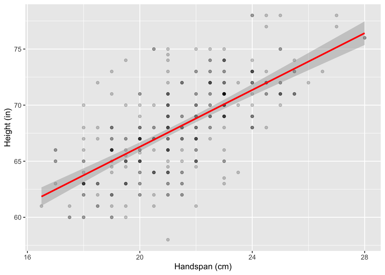

Suppose I run a simple linear regression of an outcome variable on a predictor variable. If I save the fitted values from this regression and then run a second regression of the outcome variable on the fitted values, what will I get? For extra credit: how will the R-squared from the second regression compare to that from the first regression? Example: Height and Handspan Here’s a simple example: a regression of height, measured in inches, on handspan, measured in centimeters. 1 library(tidyverse) library(broom) dat <- read_csv('https://ditraglia.com/data/height-handspan.csv') ggplot(dat, aes(y = height, x = handspan)) + geom_point(alpha = 0.2) + geom_smooth(method = "lm", color = "red") + labs(y = "Height (in)", x = "Handspan (cm)") # Fit the regression reg1 <- lm(height ~ handspan, data = dat) tidy(reg1) ## # A tibble: 2 × 5
term estimate std.error statistic p.value
## 1 (Intercept) 40.9 1.67 24.5 9.19e-76
2 handspan 1.27 0.0775 16.3 3.37e-44 As expected, bigger people are bigger in all dimensions, on average, so we see a positive relationship between handspan and height. Now let’s save the fitted values from this regression and run a second regression of height on the fitted values: dat <- reg1 |>
augment(dat) reg2 <- lm(height ~ .fitted, data = dat) tidy(reg2) ## # A tibble: 2 × 5
term estimate std.error statistic p.value
## 1 (Intercept) -1.76e-13 4.17 -4.23e-14 1.000e+ 0
2 .fitted 1.00e+ 0 0.0612 1.63e+ 1 3.37 e-44 The intercept isn’t quite zero, but it’s about as close as we can reasonably expect to get on a computer and the slope is exactly one. Now how about the R-squared? Let’s check: glance(reg1) ## # A tibble: 1 × 12
r.squared adj.r.squared sigma statistic p.value df logLik AIC BIC
## 1 0.452 0.450 3.02 267. 3.37e-44 1 -822. 1650. 1661.
# ℹ 3 more variables: deviance , df.residual , nobs glance(reg2) ## # A tibble: 1 × 12
r.squared adj.r.squared sigma statistic p.value df logLik AIC BIC
## 1 0.452 0.450 3.02 267. 3.37e-44 1 -822. 1650. 1661.
# ℹ 3 more variables: deviance , df.residual , nobs The R-squared values from the two regressions are identical ! Surprised? Now’s your last chance to think it through on your own before I give my solution. Solution Suppose we wanted to choose (\alpha_0) and (\alpha_1) to minimize (\sum_{i=1}^n (Y_i - \alpha_0 - \alpha_1 \widehat{Y}_i)^2) where (\widehat{Y}_i = \widehat{\beta}_0 + \widehat{\beta}_1 X_i) . This is equivalent to minimizing [
\sum_{i=1}^n \left[Y_i - (\alpha_0 + \alpha_1 \widehat{\beta}0) - (\alpha_1\widehat{\beta}1)X_i\right]^2. ] By construction (\widehat{\beta}0) and (\widehat{\beta}1) minimize (\sum{i=1}^n (Y_i - \beta_0 - \beta_1 X_i)^2) , so unless (\widehat{\alpha_0} = 0) and (\widehat{\alpha_1} = 1) we’d have a contradiction! Similar reasoning explains why the R-squared values for the two regressions are the same. The R-squared of a regression equals (1 - \text{SS}{\text{residual}} / \text{SS}{\text{total}}) [ \text{SS}{\text{total}} = \sum_{i=1}^n (Y_i - \bar{Y})^2,\quad \text{SS}{\text{residual}} = \sum{i=1}^n (Y_i - \widehat{Y}_i)^2 ] The total sum of squares is the same for both regressions because they have the same outcome variable. The residual sum of squares is the same because (\widehat{\alpha}_0 = 0) and (\widehat{\alpha}_1 = 1) together imply that both regressions have the same fitted values. Here I focused on the case of a simple linear regression, one with a single predictor variable, but the same basic idea holds in general. In case you don’t know what handspan is: stretch out your dominant hand, and measure from the tip of your thumb to the tip of your pinky finger. This is your handspan. I collected this dataset from many years of Econ 103 classes at UPenn. ↩︎